Today I want to talk about stream analytics, batch analytics and Apache Iceberg. Stream and batch analytics work differently but both can be built on top of Iceberg, but due to their differences there can be a tug-of-war over the Iceberg table itself. In this post I am going to use two real-world systems, Apache Fluss (streaming tabular storage) and Confluent Tableflow (Kafka-to-Iceberg), as a case study for these tensions between stream and batch analytics.
Apache Fluss uses zero-copy tiering to Iceberg. Recent data is stored on Fluss servers (using Kafka replication protocol for high availability and durability) but is then moved to Iceberg for long-term storage. This results in one copy of the data.
Confluent Kora and Tableflow uses internal topic tiering and Iceberg materialization, copying Kafka topic data to Iceberg, such that we have two copies (one in Kora, one in Iceberg).
This post will explain why both have chosen different approaches and why both are totally sane, defensible decisions.
Stream-order vs Batch-order
First we should understand the concepts of stream-order and batch-order.
A streaming Flink job typically assumes its sources come with stream-order. For example, a simple SELECT * Flink query assumes the source is (loosely) temporally ordered, as if it were a live stream. It might be historical data, such as starting at the earliest offset of a Kafka topic, but it is still loaded in a temporal order. Windows and temporal joins also depend on the source being stream-ordered to some degree, to avoid needing large/infinite window sizes which blow up the state.
A Spark batch job typically hopes that the data layout of the Iceberg table is batch-ordered, say, partitioned and sorted by business values like region, customer etc), thus allowing it to efficiently prune data files that are not relevant, and to minimize costly shuffles.
The streaming bootstrap
If Flink is just reading a Kafka topic from start to end, it’s nothing special. But we can also get fancy by reading from two data sources: one historical and one real-time. The idea is that we can unify historical data from Iceberg (or another table format) and real-time data from some kind of event stream. We call the reading from the historical source, bootstrapping.
Streaming bootstrap refers to running a continuous query that reads historical data first and then seamlessly switches to live streaming input. In order to do the switch from historical to real-time source, we need to do that switch on a given offset. The notion of a “last tiered offset” is a correctness boundary that ensures that the bootstrap and the live stream blend seamlessly without duplication or gaps. This offset can be mapped to an Iceberg snapshot.
Fig 1. Bootstrap a streaming Flink job from historical then switch to real-time.
However, if the historical Iceberg data is laid out with a batch-order (partitioned and sorted by business values like region, customer etc) then the bootstrap portion of a SELECT * will appear completely out-of-order relative to stream-order. This breaks the expectations of the user, who wants to see data in the order it arrived (i.e., stream-order), not a seemingly random one.
We could sort the data first from batch-order back to stream-order in the Flink source before it reaches the Flink operator level, but this can get really inefficient.
Fig 2. Sort batch-ordered historical data in the Flink source task.
If the table has been partitioned by region and sorted by customer, but we want to sort it by the time it arrived (such as by timestamp or Kafka offset), this will require a huge amount of work and data shuffling (in a large table). The result is not only a very expensive bootstrap, but also a very slow one (afterall, we expect fast results with a streaming query).
So we hit a wall:
Flink wants data ordered temporally for efficient streaming bootstrap.
Batch workloads want data ordered by value (e.g., columns) for effective pruning and scan efficiency.
These two data layouts are orthogonal. Temporal order preserves ingest locality; value order preserves query locality. You can’t have both in a single physical layout.
The Apache Fluss Strategy (optimize for streaming)
Fluss is a streaming tabular storage layer built for real-time analytics which can serve as the real-time data layer for lakehouse architectures. I did a comprehensive deep dive into Apache Fluss recently, diving right into the internals if you are interested.
Apache Fluss takes a clear stance. It’s designed as a streaming storage layer for data lakehouses, so it optimizes Iceberg for streaming bootstrap efficiency. It does this by maintaining stream-order in the Iceberg table.
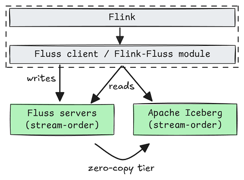
Fig 3. Fluss stores real-time and historical data in stream-order.
Internally, Fluss uses its own offset (akin to the Kafka offset) as the Iceberg sort order. This ensures that when Flink reads from Iceberg, it sees a temporally ordered sequence. The Flink source can literally stream data from Iceberg without a costly data shuffle.
Let’s take look at a Fluss log table.
A log table can define:
Optional partitioning keys (based on one or more columns). Without them, a table is one large partition.
The number of buckets per partition. The bucket is the smallest logical subdivision of a Fluss partition.
Optional bucketing key for hash-bucketing. Else rows are added to random buckets, or round-robin.
The partitioning and buckets are both converted to an Iceberg partition spec.
Fig 4. An example of the Iceberg partition spec and sort order
Within each of these Iceberg partitions, the sort order is the Fluss offset. For example, we could partition by a date field, then spread the data randomly across the buckets within each partition.
Fig 5. The partitions of an Iceberg table visualized.
Inside Flink, the source will generate one “split” per table bucket, routing them by bucket id to split readers. Due to the offset sort order, each Parquet file should contain contiguous blocks of offsets after compaction. Therefore each split reader naturally reads Iceberg data in offset order until it switches to the Fluss servers for real-time data (also in offset order).
Fig 6. Flink source bootstraps from Iceberg visualized
Once the lake splits have been read, the readers start reading from the Fluss servers for real-time data. This is great for Flink streaming bootstrap (it is just scanning the data files as a cheap sequential scan).
Primary key tables are similar but have additional limitations on the partitioning and bucketing keys (as they must be subsets of the primary key). A primary key, such as device_id, is not a good partition column as it’s too fine grained, leading us to use an unpartitioned table.
Fig 7. Unpartitioned primary key table with 6 buckets.
If we want Iceberg partitioning, we’ll need to add another column (such as a date) to the primary key and then use the date column for the partitioning key (and device_id as a bucket key for hash-bucketing). This makes the device_id non-unique though.
In short, Fluss is a streaming storage abstraction for tabular data in lakehouses and stores both real-time and historical data in stream-order. This layout is designed for streaming Flink jobs. But if you have a Spark job trying to query that same Iceberg table, pruning is almost useless as it does not use a batch-optimized layout. Fluss may well decide to support Iceberg custom partitioning and sorting (batch-order) in the future, but it will then face the same challenges of supporting streaming bootstrap from batch-ordered Iceberg.
The Confluent Tableflow Strategy
Confluent’s Tableflow (the Kafka-to-Iceberg materialization layer) took the opposite approach. It stores two copies of the data: one stream-ordered and one optionally batch-ordered.
Kafka/Kora internally tiers log segments to object storage, which is a historical data source in stream-order (good for streaming bootstrap). Iceberg is a copy, which allows for stream-order or batch-order, it’s up to the customer. Custom partitioning and sort order is not yet available at the time of writing, but it’s coming.
Fig 8. Tableflow continuously materializes a copy of a Kafka topic as an Iceberg table.
I already wrote why I think zero-copy Iceberg tiering is a bad fit for Kafka specifically. Much also applies to Kora, which is why Tableflow is a separate distributed component from Kora brokers.
So if we’re going to materialize a copy of the data for analytics, we have the freedom to allow customers to optimize their tables for their use case, which is often batch-based analytics.
Fig 9. Copy 1 (original): Kora maintains stream-ordered live and historical Kafka data. Copy 2 (derived): Tableflow continuously materializes Kafka topics as Iceberg tables.
If the Iceberg table is also stored in stream-order then Flink could do an Iceberg streaming bootstrap and then switch to Kafka. This is not available right now in Confluent, but it could be built. There are also improvements that could be made to historical data stored by Kora/Kafka, such as using a columnar format for log segments (something that Fluss does today).
Either way, the materialization design provides the flexibility to execute a streaming bootstrap using a stream-order historical data source, allowing the customer to optimize the Iceberg table according to their needs.
Conclusions
Batch jobs want value locality (data clustered by common predicates), aka batch-order. Streaming jobs want temporal locality (data ordered by ingestion), aka stream-order. With a single Iceberg table, once you commit to one, the other becomes inefficient.
Given this constraint, we can understand the two different approaches:
Fluss chose stream-order in its Iceberg tables to support stream analytics constraints and avoid a second copy of the data. That’s a valid design decision as after all, Fluss is a streaming tabular storage layer for real-time analytics that fronts the lakehouse. But it does mean giving up the ability to use Iceberg’s layout levers of partitioning and sorting to tune batch query performance.
Confluent chose a stream-order in Kora and one optionally batch-ordered Iceberg copy (via Tableflow materialization), letting the customer decide the optimum Iceberg layout. That’s also a valid design decision as Confluent wants to connect systems of all kinds, be they real-time or not. Flexibility to handle diverse systems and diverse customer requirements wins out. But it does require a second copy of the data (causing higher storage costs).
As the saying goes, the opposite of a good idea can be a good idea.
It all depends on what you are building and what you want to prioritize. The only losing move is pretending you can have both (stream-optimized and batch-optimized workloads) in one Iceberg table without a cost. Once you factor in the compute cost of using one format for both workloads, the storage savings disappear. If you really need both, build two physical views and keep them in sync.
Some related blog posts that are relevant this one: